PyTorch coding: a binary classification example

A step by step tutorial for binary classification with PyTorch

Aug 27, 2021 by Xiang Zhang

In this blog, I would like to share with you how to solve a simple binary classification problem with neural network model implemented in PyTorch. First, let's look at the problem.

import numpy as np
import matplotlib.pyplot as plt
from sklearn.datasets import make_classification
X, Y = make_classification(n_features=2, n_redundant=0, n_clusters_per_class=1)
plt.scatter(X[:, 0], X[:, 1], c=Y,cmap='jet')
                

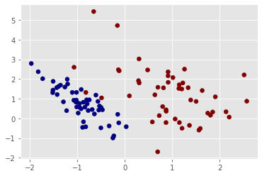
Data is loaded from scikit-learn package. What we will do is to find a decision boundary to separate these dots of two different colors. As you can see, these two sets of dots are linearly separable in two dimensions. Constructing the classifier model as a single layer neural network with a sigmoid activation function would be sufficient. We use dots coordinates as inputs, dots classes as ground truths. Loss function is the binary cross entropy of predicted class and ground truth class.

import torch
model = torch.nn.Sequential(
    torch.nn.Linear(2, 1),
    torch.nn.Sigmoid(),
)
params = list(model.parameters())
x = torch.from_numpy(X.astype(np.float32))
y = torch.from_numpy(Y.astype(np.float32)).view(-1,1)
loss_fn = torch.nn.BCELoss()
            

Let the training begin. At every training step, we set the accumulated gradients to zero, calculate the loss, propagate it backwards to get new gradients(derivative chain), update the model weights.

learning_rate = 1e-1
loss_list = []
for t in range(1000):
    y_pred = model(x)
    loss = loss_fn(y_pred, y)
    loss_list.append(loss.item())
    model.zero_grad()
    loss.backward()
    with torch.no_grad():
        for param in model.parameters():
            param -= learning_rate * param.grad
            

After that, we visualize the loss curve.

step = np.linspace(0,1000,1000)
plt.plot(step,np.array(loss_list))
            

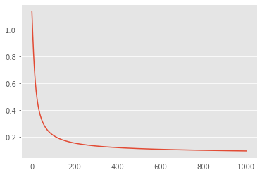
The loss curve looks converged. Finally we plot the decision boundary.

w = params[0].detach().numpy()[0]
b = params[1].detach().numpy()[0]
plt.scatter(X[:, 0], X[:, 1], c=y,cmap='jet')
u = np.linspace(X[:, 0].min(), X[:, 0].max(), 2)
plt.plot(u, (0.5-b-w[0]*u)/w[1])
plt.xlim(X[:, 0].min()-0.5, X[:, 0].max()+0.5)
plt.ylim(X[:, 1].min()-0.5, X[:, 1].max()+0.5)
            

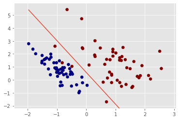
It looks good. But to evaluate the model's generalization to unseen data, we need to split dataset to training, validation and test set. We will discuss them in a future blog.

Summary

In this blog, we constructed a simple neural network and a training procedure using basic PyTorch code to solve a binary classification problem. I hope you like it. Thanks for reading.