Simple Understanding of Kinematic Bicycle Model

Explain basic 2D bicycle model step by step

Nov 14, 2021 by Yan Ding

1. Introduction

2D bicycle model can be expressed as a simplified car model. This is a classic model that does very well at capturing vehicle motion in normal driving conditions.

The bicycle model we'll develop is called the front wheel steering model, as the front wheel orientation can be controlled relative to the heading of the vehicle. The rear wheel orientation cannot be controlled. It only follows the front wheel. Our target is to compute state [x, y, θ, δ], θ is heading angle, δ is steering angle. The inputs are [ν, φ], ν is velocity, φ is steering rate.

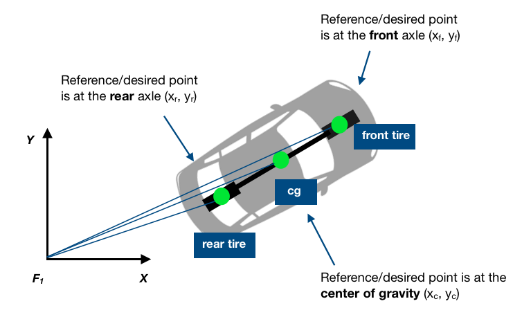
To analyze the kinematics of the bicycle model, we must select a reference point (X, Y) on the vehicle which can be placed at the center of the rear axle, the center of the front axle, or at the center of gravity or cg.

2. Model Analysis

We know the vehicle or bicycle is a rigid body.

1. If the desired point is at the center of the rear axle, we can draw below illustration picture:


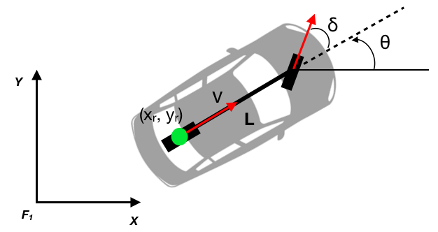
θ is heading angle, δ is steering angle.

Next to apply the Instantaneous Center of Rotation ( ICR ).



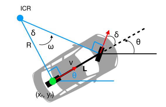
In order to get the state change [x, y, θ, δ], we need first compute the state change rate: [x_dot, y_dot, θ_dot, δ_dot].

x_dot = v * cos(θ)

y_dot = v * sin(θ)

θ_dot = ω, ω is rotation rate.

ω = ν / R, R is radius.

We need first know how to compute R. As the figure above shows, L is the bicycle length, δ is steering angle, so R can be computed as:

R = L / tan(δ)

So we can arrive:

θ_dot = ν / (L / tan(δ)) = ν * tan(δ) / L

δ_dot = φ (φ is the input: the rate of change of steering angle).

To summarize, the state change rate [x_dot, y_dot, θ_dot, δ_dot] is:

[v * cos(θ), v * sin(θ), ν * tan(δ)/L, φ]



2. If the desired point is at the center of the front axle:


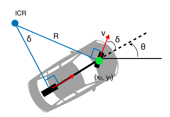
As figure above shows, desired point is in the center of front wheel. We can arrive:

R = L / sin(δ).

So We can get the changing rate [x_dot, y_dot, θ_dot, δ_dot] as following:

x_dot = v * cos(δ + θ)

y_dot = v * sin(δ + θ)

θ_dot = v / R = v / (L/sin(δ)) = v * sin(δ)/L

δ_dot = φ

To summarize, the state change rate is:

[v * cos(δ + θ), v * sin(δ + θ), ν * sin(δ)/L, φ]



3. If the desired point is at the center of gravity or cg, we can have following figure:


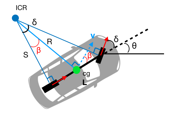
β is the slip angle. According to the illustrated image, we can arrive following equations:

x_dot = v * cos(β + θ)

y_dot = v* sin(β + θ)

This model is a little complicated. We need first compute R in order to get θ_dot. As shown in figure above, we can first compute S.

S = L / tan(δ)

Then we can use S and β angle to compute R.

R = S / cos(β) = L / (tan(δ) *cos(β))

As we know R now, we can get θ_dot as following:

θ_dot = v / R = v *tan(δ) *cos(β) / L

Furthermore, if we know the distance between the rear wheel and cg denoted as l_r, we can also compute the slip angle β.



tan(β) = l_r / S = l_r /(L / tan(δ)) = l_r * tan(δ) / L

So slip angle β = arctan(l_r * tan(δ) / L)

Changing rate of steering angle is: δ_dot = φ

To summarize, the state change rate is:

[v * cos(β + θ), v* sin(β + θ), v *tan(δ) *cos(β), φ] , where β = arctan(l_r * tan(δ) / L)

3. Summary

To recap, our model is the bicycle kinematic model as has been analyzed. States(outputs) are[x, y, θ, δ]. Inputs are [ν, φ], ν is velocity, φ is steering rate. We can compute the changing rate of [x, y, θ, δ], which is x_dot, y_dot, θ_dot, δ_dot. To get the final state [x, y, θ, δ], we can use discrete time model.

x_(t+1) = x_t + x_dot * Δt

y_(t+1) = y_t + y_dot * Δt

θ_(t+1) = θ_t + θ_dot * Δt

δ_(t+1) = δ_t + δ_dot * Δt